|
 |
 |
 |


Technical Report D:
Management templates
for increased biodiversity and economics in intensively managed loblolly
pine plantations
Final Technical Report to the National Commission on Science for Sustainable Forestry (NCSSF)July 31, 2005 Kevin W. Zobrist Michael G. Andreu Thomas M. Hinckley Kevin R. Gehringer Craig W. Hedman The National Commission on Science for Sustainable Forestry (NCSSF) sponsored the research described in this report. The National Council on Science and the Environment (NCSE) conducts the NCSSF program with support from the Doris Duke Charitable Foundation, the David and Lucile Packard Foundation, the Surdna Foundation, and the National Forest Foundation.
ContentsBack to Main Report
I. IntroductionThere are a number of stand-level management practices that can support increased biodiversity in intensively managed loblolly pine (Pinus taeda) plantations.1 These practices include thinning, prescribed burning, less intensive site preparation, longer rotations, and others (for a complete review see Zobrist et al. 2005b). For best results, many of these practices can be used in combination with each other, though timing is important. For landowners or managers interested in supporting greater biodiversity in their plantations, it can be useful to summarize these practices into a set of specific but flexible guidelines or management “templates.” From a private landowner’s perspective, it is particularly useful to identify templates that will support increased biodiversity while maintaining an acceptable economic return. Some practices for increasing biodiversity are complimentary with timber production and economic goals, while others involve some level of trade-off (Allen et al. 1996, Hunter 1990). An approach for creating templates for achieving biodiversity and economic goals has been developed for riparian zone management in the Pacific Northwest (Zobrist et al. 2004, 2005a, 2005c). Using this approach, we have developed an example template for southern loblolly pine plantations as a demonstration of how the approach developed in the Pacific Northwest can be used to address biodiversity issues in other regions. In this report we will describe how the template approach was applied to southern conditions, examine the biodiversity and economic outcomes of the example template, and discuss additional southern applications of this template process.
|
||||||||||||||||||||||||||||||||||||||||||||||||||||||||||||||||||||||||||||||||||||||||||||||||||||||||||||||||||||||||||||||||||||||||||||||||||||||||||||||||||||||||||||||||||||||||||||||||||||||||||||||||||||||||||||||||||||||||||||||||||||||||||||||||||||||||||||||||||||||||||||||||||||||||||||||||||||||||||||||||||||||||||||||||||||||||||||||||||||||||||||||||||||||||||||||||||||||||||||||||||||||||||||||||||||||||||||||||||||||||||||||||||||||||||||||||||||||||||||||||||||||||||||||||||||||||||||||||||||||||||||||||||||||||||||||||||||||||||||||||||||||||||||||||||||||||||||||
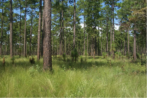 |
| Figure 1: An example of the benchmark conditions measured at International Paper’s Southlands Forest (stand 400-053) by Hedman et al. (2000). The open, park-like structure of this uneven-aged longleaf pine-wiregrass stand supports a rich, herbaceous understory that provides habitat for a wide range of game and non-game wildlife species. Photograph taken by Craig Hedman. |
Four key structural attributes were identified from the benchmark plot dataset: the density in trees per acre (TPA) and the quadratic mean diameter (QMD) of larger trees, and the density and QMD of smaller trees. Trees with a diameter at breast height (DBH) greater than 8 inches were considered larger trees, and those less than 8 inches in DBH were considered small trees.3 The distributions of values for these four attributes when considered at the same time may be used to create a four-dimensional target region. The four-dimensional target can be represented visually by splitting the large tree and small tree density and QMD components into sub-targets that can be plotted in two dimensions (Figure 2). The elliptical region in each sub-target represents an approximate 95% acceptance level, and this is the region that encompasses the central 95% of the target data, assuming a normal distribution. By using only the central 95% of the target, the influence of the most extreme outlying values in the target dataset are reduced. An observed stand structure that simultaneously falls within these two elliptical sub-target regions is statistically similar to the benchmark plots.
![]()
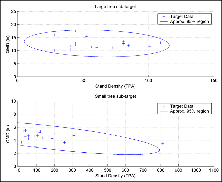 |
| Figure 2: The 4-dimensional stand structure target is split into larger tree and smaller tree stand density and QMD sub-targets that can each be plotted visually in two dimensions. The ellipses represent approximate 95% acceptance regions for each sub-target. When comparing this target data to the one for Douglas-fir (see Zobrist et al. 2005c), the limitations of the pine dataset become clear as there are few data points outside of the 95% acceptance area. |
The four-dimensional target provides a high degree of discrimination between the benchmark and non-benchmark plots. By including both a larger tree and a smaller tree component in the target, we can assess stands to make sure that they have an open pine canopy but have not developed a dense midstory. To be in the target, an observed stand must have some larger trees, but not too many or too few, while also having smaller trees in a midstory or understory, but again not too many or too few. The percent time over a 100-year simulation that predicted stand structures fall within the 95% target region was used as a specific biodiversity criterion for assessing potential template.
There are several metrics that can be used as economic performance criteria. Soil expectation value (SEV), or bare land value, is the net present value of a complete forest rotation repeated in perpetuity given a target rate of return (Klemperer 1995). This is perhaps the most important single economic criterion, as it reflects the economic performance of the initial investment in establishing a plantation given an expected management regime. This will be the metric of most relevance for landowners implementing a template that starts from bare land.
SEV is also relevant for landowners starting with mid-rotation stands, as at some point they will reach rotation end and be faced with the decision of whether or not to continue the template for additional rotations. Thus, SEV is the best indicator of long-term economic acceptability. However, landowners with mid-rotation stands may also be interested in the overall forest value (FV), which is also known as land and timber value (Klemperer 1995). FV includes SEV along with the net present value of the expected costs and revenues to hold the existing timber through the end of the current rotation, including the opportunity cost of using the land. In developing templates, we used SEV as the primary economic criterion but also considered FV for mid-rotation stands. In both cases, 5% was used as the target real rate of return, which is typical for financial analysis calculations.
![]()
III. Simulating management alternatives
The next step in developing templates is to define potential management alternatives. We established nine different alternatives that were intended to represent a range of management prescriptions that a private landowner might use if intending to harvest a minimum of some small sawtimber (chip and saw) at the end of the rotation. The first alternative was a 25-year chip and saw rotation, while the other eight were sawtimber rotations ranging from 35 to 55 years. Each alternative included a commercial thinning at age 15 in which every 5th row was removed, along with additional thinning from below to remove a total of 30% of the stand volume.
The sawtimber rotations included subsequent thinnings from below starting at age 25. To balance the frequency needed to maintain an open canopy with the economic viability of the operation, we used thinning intervals of either 10 or 15 years. We used two different thinning intensities, leaving a residual basal area (BA) of either 60 or 80 ft2/acre. The complete list of alternatives is below. Table 1 shows a management timeline of each alternative.
- 25-year chip and saw rotation
- 35-year sawtimber rotation with 10-year thinning interval to 60 ft2/acre BA
- 35-year sawtimber rotation with 10-year thinning interval to 80 ft2/acre BA
- 40-year sawtimber rotation with 15-year thinning interval to 60 ft2/acre BA
- 40-year sawtimber rotation with 15-year thinning interval to 80 ft2/acre BA
- 55-year sawtimber rotation with 10-year thinning interval to 60 ft2/acre BA
- 55-year sawtimber rotation with 10-year thinning interval to 80 ft2/acre BA
- 55-year sawtimber rotation with 15-year thinning interval to 60 ft2/acre BA
- 55-year sawtimber rotation with 15-year thinning interval to 80 ft2/acre BA
| Alt | Year |
||||||||
15 |
20 |
25 |
30 |
35 |
40 |
45 |
50 |
55 |
|
1 |
Thin 30% |
Clear-cut |
|||||||
2 |
Thin 30% |
Thin 60 BA |
Clear-cut |
||||||
3 |
Thin 30% |
Thin 80 BA |
Clear-cut |
||||||
4 |
Thin 30% |
Thin 60 BA |
Clear-cut |
||||||
5 |
Thin 30% |
Thin 80 BA |
Clear-cut |
||||||
6 |
Thin 30% |
Thin 60 BA |
Thin 60 BA |
Thin 60 BA |
Clear-cut |
||||
7 |
Thin 30% |
Thin 80 BA |
Thin 80 BA |
Thin 80 BA |
Clear-cut |
||||
8 |
Thin 30% |
Thin 60 BA |
Thin 60 BA |
Clear-cut |
|||||
9 |
Thin 30% |
Thin 80 BA |
Thin 80 BA |
Clear-cut |
|||||
![]()
Each management alternative was simulated using the Landscape Management System (LMS). LMS provides a user-friendly interface that integrates existing and publicly available growth, treatment, and visualization models (McCarter et al. 1998). One of the growth models that LMS interfaces with is the USDA Forest Service’s Forest Vegetation Simulator (FVS). For our simulations we used the Southern Variant of FVS (Donnelly et al. 2001, Stage 1973, Wykoff et al. 1982).
Simulations were begun on a representative inventory from a 10-year-old plantation that was one of the benchmark plots (stand 300-030). The 25-year site index was 55. To be compatible with LMS, we converted this to a 50-year site index of 73 using a factor of 1.32 (North Carolina Division of Forest Resources 1988). We further increased the site index to 80 in the growth model to account for intensive management practices (Siry et al. 2001).
For each thinning operation, it was assumed that in addition to thinning the crop trees, all non-crop trees over 5 inches DBH were removed except for a small component (13 TPA) of desirable, mast-producing hardwoods (black cherry, hickory, and various oaks). For trees under 5 inches DBH, 40% of the stems were removed at the time of thinning to simulate mortality from being crushed, etc. during the operation. In the absence of understory vegetation control, heavy, repeated thinnings can result in an undesirable hardwood midstory that inhibits the understory (Hunter 1990, Schultz 1997). For our simulations, we assumed that prescribed burning was done every 5 years starting at age 20. This was not directly represented in our simulations. Rather, the impacts of burning on understory tree composition were indirectly represented by not simulating the natural hardwood ingrowth that would be expected after thinning treatments, assuming that such ingrowth would be killed or suppressed by burning.
Using LMS projections, stand structure relative to the target conditions can be assessed over time. Economic metrics for each alternative can be computed using an integrated financial analysis program called Economatic. An imbedded bucking algorithm is used to divide harvested trees into different log sorts based on user-defined parameters. User-defined log prices are then applied, and revenue calculations are imported into Economatic. Economatic then applies additional user-defined costs and revenues (such as planting and prescribed burning costs) and calculates both SEV and FV.
For these simulations, we used 1st quarter 2005 average stumpage prices for Georgia Region 2 (Timber Mart-South 2005). Since LMS volume outputs were in cubic feet, we converted board foot prices to cubic foot prices using a factor of 5 board feet/cubic foot (North Carolina Division of Forest Resources 1988). Prices per cord were converted using a factor of 75 cubic feet/cord (Timber Mart-South 2005). Cost assumptions included $13.25/acre for prescribed burning (Dubois et al. 2003) and $8/acre annual property taxes and overhead costs (Siry 2002). SEV was calculated retrospectively by assuming a $215/acre cost for planting and site preparation (Dubois et al. 2003, Siry 2002) at the beginning of the rotation (10 years prior to the beginning of the simulations on the 10-year-old representative inventory). All financial calculations were done before income taxes.
![]()
IV. Results
The percent time in target over a 100-year simulation, along with SEV/acre and FV/acre, is summarized for each alternative in Table 2. Alternative 1, the 25-year chip and saw rotation, never achieved structure similar to the target; it also had the lowest economic performance. SEV for this alternative was negative, indicating that, given our assumptions, investing in this rotation would not earn the target real rate of return of 5%. Shorter rotations generally have favorable economic returns. Our results may reflect several factors. The growth model computes volume based on a minimum 4-inch top, which can underestimate the volume of small-diameter pulp and chip and saw logs. The historically low current pulp price ($18.40/cord) was also a likely factor.
FV figures are higher than SEV, as they include the existing 10-year-old inventory for which establishment costs are sunk. The 35 and 45-year rotations (Alternatives 2-5) reached the target less than 25% of the time, but tended to perform well economically, with Alternative 5 performing the best. The 55-year rotations (Alternatives 6-9) had the most time in the target and had moderate economic performance. The stumpage values used to compute SEV and FV, along with harvested volume, are summarized in Table 3 and Table 4 respectively.
| Table 2: Comparison of time in target over 100 years, SEV/acre, and FV/acre for each alternative. |
Alternative |
% Time in Target |
SEV/Acre |
FV/Acre |
1 |
0% |
($20) |
$418 |
2 |
14% |
$423 |
$1,140 |
3 |
14% |
$480 |
$1,233 |
4 |
24% |
$466 |
$1,210 |
5 |
14% |
$619 |
$1,459 |
6 |
48% |
$305 |
$947 |
7 |
48% |
$413 |
$1,124 |
8 |
48% |
$382 |
$1,074 |
9 |
38% |
$415 |
$1,127 |
![]()
| Table 3: Total harvest revenue by year for each alternative. |
| Alternative | Year |
||||||||
15 |
20 |
25 |
30 |
35 |
40 |
45 |
50 |
55 |
|
1 |
$107 |
$905 |
|||||||
2 |
$107 |
$375 |
$2,990 |
||||||
3 |
$107 |
$263 |
$3,432 |
||||||
4 |
$107 |
$375 |
$4,253 |
||||||
5 |
$107 |
$263 |
$5,412 |
||||||
6 |
$107 |
$375 |
$634 |
$755 |
$4,477 |
||||
7 |
$107 |
$263 |
$746 |
$1,206 |
$5,408 |
||||
8 |
$107 |
$375 |
$1,656 |
$5,004 |
|||||
9 |
$107 |
$263 |
$1,750 |
$5,741 |
|||||
| Table 4: Total harvested volume (cubic feet) by year for each alternative. |
Alternative |
Year |
||||||||
15 |
20 |
25 |
30 |
35 |
40 |
45 |
50 |
55 |
|
1 |
435 |
2,965 |
|||||||
2 |
435 |
1,533 |
2,439 |
||||||
3 |
435 |
1,073 |
3,141 |
||||||
4 |
435 |
1,533 |
2,973 |
||||||
5 |
435 |
1,073 |
3,772 |
||||||
6 |
435 |
1,533 |
721 |
518 |
2,526 |
||||
7 |
435 |
1,073 |
896 |
758 |
3,289 |
||||
8 |
435 |
1,533 |
1,158 |
2,918 |
|||||
9 |
435 |
1,073 |
1,409 |
3,593 |
|||||
![]()
For each alternative, the simulation cycles that achieved the target conditions are shaded in Table 5. This gives some insight as to which management strategies were most successful in producing target structures. All of the sawtimber rotations reached the target after the second commercial thinning. All of the alternatives that were thinned to 60 ft2/acre of BA remained in the target until final harvest, as did those that were thinned to 80ft2/acre of BA at 10-year intervals. When thinned to 80ft2/acre at 15-year intervals (Alternative 9), the stand fell out of the target 10 years after the second thinning. This suggests that heavier or more frequent thinnings are necessary to maintain the target structure. The alternatives in which thinning was done to 80 ft2/acre (3,5,7,9) produced a better economic return than the comparable alternatives that were thinned to 60ft2/acre (2,4,5,8). Thus, thinning more frequently to 80 ft2/acre might be a good way to balance objectives. In each case, the overall time in target was limited by the rotation age.
| Table 5: The management timelines from Table 1 with shaded areas indicating the simulation cycles for which the target conditions were achieved. |
| Alt | Year |
||||||||
15 |
20 |
25 |
30 |
35 |
40 |
45 |
50 |
55 |
|
1 |
Thin 30% |
Clear-cut |
|||||||
2 |
Thin 30% |
Thin 60 BA |
Clear-cut |
||||||
3 |
Thin 30% |
Thin 80 BA |
Clear-cut |
||||||
4 |
Thin 30% |
Thin 60 BA |
Clear-cut |
||||||
5 |
Thin 30% |
Thin 80 BA |
Clear-cut |
||||||
6 |
Thin 30% |
Thin 60 BA |
Thin 60 BA |
Thin 60 BA |
Clear-cut |
||||
7 |
Thin 30% |
Thin 80 BA |
Thin 80 BA |
Thin 80 BA |
Clear-cut |
||||
8 |
Thin 30% |
Thin 60 BA |
Thin 60 BA |
Clear-cut |
|||||
9 |
Thin 30% |
Thin 80 BA |
Thin 80 BA |
Clear-cut |
|||||
![]()
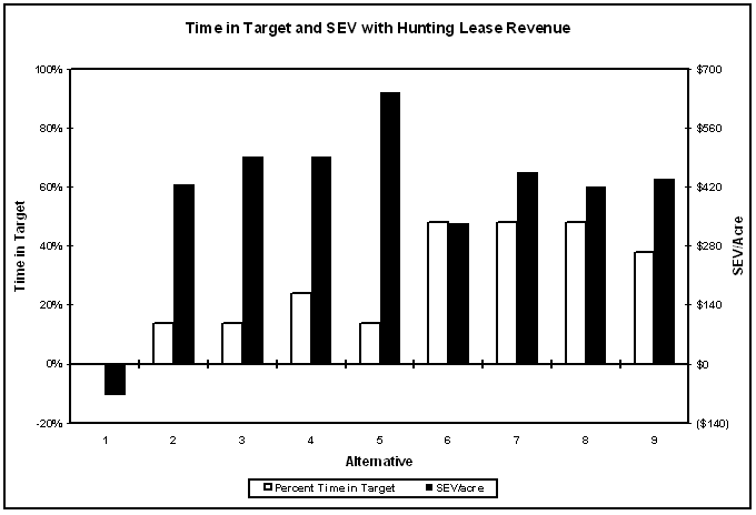
Aside from Alternative 1, which performed the worst relative to both criteria, increasing the percent time in target will involve some level of economic trade-off relative to Alternative 5, which had the highest SEV. The performance of each alternative relative to the two primary template criteria, time in target and SEV, are plotted in Figure 3 to show a visual comparison of the trade-offs.
As shown in Figure 3, maximizing the time in target (Alternatives 6-8) involves a trade-off with SEV. One way this trade-off might be minimized is through increased hunting lease revenue. Hunting leases can provide forest landowners in the South with significant supplemental revenue, especially for landowners who provide high-quality habitat (Baker and Hunter 2002, Johnson 1995, Jones et al. 2001). Using time in target as an indicator of habitat quality, landowners who provide more time in target may earn hunting lease premiums. Figure 4 shows what the relative trade-offs for each alternative would be assuming the following hunting lease rates: $4/acre for less than 20% time in target, $8/acre for 20-40% time in target, and $12/acre for greater than 40% time in target.4 The trade-offs still exists, but they are reduced for the alternatives that have the most time in target, which may make these costlier alternatives more acceptable to private landowners.
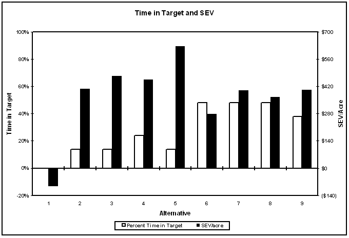 |
| Figure 3: The percent time in target over 100 years plotted together with the SEV/acre for each alternative illustrates some of the trade-offs between biodiversity and economic return. |
![]()
Quantifying the trade-offs between time in target and SEV can help identify the best template options from our 9 alternatives. Table 6 summarizes the SEV cost (assuming hunting lease premiums) for each alternative as the difference relative to the maximum possible (Alternative 5). Both the total cost and the cost per percent time in target are given.
Three alternatives emerged from Table 4, illustrating a range of template options. The lowest cost template would be Alternative 5, for landowners who want to provide some level of biodiversity but not sacrifice economics. Of the alternatives that provided a higher percent of time in target, Alternative 4 was the lowest cost alternative and may be desirable for landowners who want to make a small improvement in biodiversity but cannot afford significant costs. Alternative 7 had the lowest overall cost/benefit ratio and thus produced the desired structure most efficiently. For supporting significantly increased biodiversity while maintaining a competitive economic performance, this may be the overall most desirable template option. Figure 5 illustrates the projected stand development from age 10 to 55 under Alternative 7. Complete stand development projections for each alternative are shown in the Appendix.
 |
| Figure 4: The percent time in target over 100 years plotted together with the SEV/acre for each alternative assuming hunting lease premiums, which can reduce economic trade-offs for alternatives with high time in target scores. |
![]()
| Table 6: Comparison of the SEV costs (as the difference relative to the maximum possible) and percent time in target over 100 years for each alternative. |
Alternative |
% Time in Target |
SEV/Acre |
SEV Cost |
Cost/% in target |
1 |
0% |
($2) |
$639 |
N/A |
2 |
14% |
$442 |
$195 |
$13.93 |
3 |
14% |
$499 |
$138 |
$9.86 |
4 |
24% |
$503 |
$134 |
$5.58 |
5 |
14% |
$637 |
$0 |
$0 |
6 |
48% |
$360 |
$277 |
$5.77 |
7 |
48% |
$469 |
$168 |
$3.50 |
8 |
48% |
$438 |
$199 |
$4.15 |
9 |
38% |
$452 |
$185 |
$4.87 |
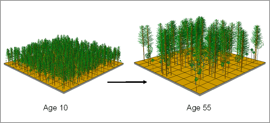 |
| Figure 5: Projected stand development from age 10 to 55 under Alternative 7. |
![]()
V. Template applications
The thinning and burning regime of Alternative 7 (Table 7) can potentially support significantly increased biodiversity in intensively managed loblolly pine plantations. When implementing such a template, several guidelines should be considered. One of the most important considerations is land use history. Old-field sites lack seed- and rootstock-banks (Baker and Hunter 2002). Plantations established on these sites are unlikely to develop a diverse, productive understory regardless of overstory management (Hedman et al. 2000). Thus, templates like this should only be applied to plantations established on cutover lands. Plantations on old field sites may be best managed for maximum timber production, as these sites will not likely support high levels of biodiversity.
| Table 7: Thinning and burning timeline for Alternative 7. |
Year |
15 |
20 |
25 |
30 |
35 |
40 |
45 |
50 |
55 |
| Alt 7 | Thin 30% |
Thin 80 BA |
Thin 80 BA |
Thin 80 BA |
Clear-cut |
||||
burn |
burn |
burn |
burn |
burn |
burn |
burn |
burn |
Additional management practices can be used in conjunction with a template like this to promote increased biodiversity. Moderate intensity site preparation may provide a reasonable balance of understory diversity and cost effectiveness (Locascio et al. 1990). Fertilization can promote biodiversity by improving understory food production in thinned stands (Hunter 1990, Hurst and Warren 1982). Snags and downed wood provide important habitat structures that should be retained as much as possible (Allen et al. 1996, Dickson and Wigley 2001, Lohr et al. 2002). Retaining riparian buffers will also promote biodiversity (Baker and Hunter 2002, Dickson and Wigley 2001).
Site specific factors should be taken into account when considering the frequency and timing of burning. Some suggest in general to burn before thinning, as it makes thinning easier (Hurst et al. 1980) and there will not be heavy fuel loads at the time of burning to cause the fire to burn too hot (Van Lear et al. 2004). When possible and practical, varying the season and frequency of prescribed burning can increase diversity and favor a broader suite of species (Robbins and Myers 1992). Likewise, leaving patches of unburned areas can favor some wildlife (Landers 1987, Moorman 2002). For both thinning and burning, mast-producing hardwoods like hickories and oaks should be retained if possible to provide food for wildlife (Johnson et al. 1975, Melchiors 1991).
![]()
The template presented above is just one example management strategy for supporting increased biodiversity while maintaining viable economics. The template incorporates some key basic principles for increasing biodiversity, such as longer rotations, early and frequent thinning, and prescribed burning. There are many possible variations of this proposed template that could achieve as good or better results. In particular, even longer rotations may provide for greater biodiversity. The time in target scores for the alternatives that we examined were ultimately limited by rotation length. SEV values for some of the 55-year alternatives were still competitive, especially if hunting lease premiums were assumed. Rotations longer than that can likely still achieve acceptable economic returns and may be desirable for landowners who are willing to incur additional costs to support higher levels of biodiversity. Earlier, more frequent, or heavier thinnings may also achieve target conditions sooner than the alternatives that we examined.
Most importantly, the template presented above successfully demonstrates an approach for developing sustainable management solutions that support increased biodiversity while maintaining economic viability. With additional data to quantify the desired conditions, a more robust target can be developed, which will be helpful for further refining this example template and generating additional templates. Ultimately a spectrum of management templates is needed to be applicable to a wide range of site conditions and to give landowners choices as they balance biodiversity and economic objectives.
Acknowledgements
The authors would like to acknowledge James McCarter, Kevin Ceder, and Larry Mason at the Rural Technology Initiative, University of Washington, for their contributions to this project in guidance and technical support.
Metric equivalents
| When you know: | Multiply by: | To find: |
| Cubic feet (ft3) | 0.0283 | Cubic meters |
| Feet (ft) | 0.3048 | Meters |
| Inches (in) | 2.54 | Centimeters |
| Square feet per acre (ft2/ac) | 0.229 | Square meters per hectare |
| Trees per acre (TPA) | 2.471 | Trees per hectare |
![]()
Literature cited
- Allen, A.W., Bernal, Y.K., and R.J. Moulton. 1996. Pine
plantations and wildlife in the Southeastern United States:
an assessment
of impacts and opportunities. U. S. Dept. of the Interior,
National Biological Service, Information and Technology Report
3. 32 p.
Available online at http://www.nwrc.usgs.gov/wdb/pub/others/1996_03.pdf;
last accessed June 2005.
- Baker, J.C. and W.C. Hunter. 2002. Effects of forest management
on terrestrial ecosystems. Pages 91-112 in D.N. Wear and
J.G. Greis, eds. Southern Forest Resource Assessment. General
Technical
Report SRS-53. USDA Forest Service, Southern Research Station,
Ashville, NC.
- Dickson, J.G. and T.B. Wigley. 2001. Managing forests for
wildlife. Pages 83-94 in Dickson, J.G., ed. Wildlife of
Southern Forests:
Habitat and Management. Hancock House Publishers, Blaine,
WA.
- Donnelly, D., B. Lilly, and E. Smith. 2001. The southern
variant of the Forest Vegetation Simulator. USDA Forest Service,
Forest
Management Service Center, Fort Collins, CO. 61 p. Available
online at http://www.fs.fed.us/pub/fmsc/ftp/fvs/docs/overviews/snvar.pdf;
last accessed July 2005.
- Dubois, M.R., T.J. Straka, S.D. Crim, and L.J. Robinson.
2003. Costs and cost trends for forestry practices in the South.
Forest
Landowner 62(2):3-9.
- Gehringer, K.R. In press. A nonparametric method for
defining and using biologically based targets in forest management.
In: M. Bevers, T.M. Barrett, eds. Systems Analysis in Forest
Resources:
Proceedings of the 2003 Symposium. General Technical Report
PNW-GTR-xxx. USDA Forest Service, Pacific Northwest Research
Station, Portland,
OR.

- Harris, L.D., D.H. Hirth, and W.R. Marion. 1979. The development
of silvicultural systems for wildlife. Pages 65-80 in C.L.
Shilling and J.R. Toliver, eds. Recreation in the South’s
third forest. Twenty-eighth Annual Forestry symposium, Louisiana
State
University, Baton Rouge.
- Hedman, C.W., S.L. Grace, and S.E. King. 2000. Vegetation
composition and structure of southern coastal plain pine forests:
an ecological
comparison. Forest Ecology and Management 134:233-247.
- Hunter, M.L., Jr. 1990. Wildlife, forests, and forestry:
Principles of managing forests for biological diversity. Prentice
Hall,
Englewood Cliffs, N.J. 370 p.
- Hurst, G.A., J.J. Campo, and M.B. Brooks. 1980. Deer forage
in a burned and burned-thinned pine plantation. Proceedings
of the Annual Conference of the Southeastern Association of
Fish
and Wildlife Agencies 34:476-481.
- Hurst, G.A. and R.C. Warren. 1982. Impacts of silvicultural
practices in loblolly pine plantations on white-tailed deer
habitat. Pages 484-487 in E.P. Jones, ed. Proceedings of
the second biennial
Southern Silvicultural Research Conference. General Technical
Report SE-24. USDA Forest Service, Southeastern Forest Experiment
Station, Asheville, NC.
- Johnson, A.S., J.L. Landers, and T.D. Atkeson. 1975. Wildlife
in young pine plantations. Pages 147-159 in Proceedings
of the symposium on management of young pines. USDA Forest Service,
Southeast Area, State and Private Forestry, Atlanta, GA.
- Johnson, R. 1995. Supplemental sources of income for southern
timberland owners. Journal of Forestry 93(3):22-24.
- Jones, W.D., U.A. Munn, S.C. Grado, and J.C. Jones. 2001.
Fee hunting—An income source for Mississippi’s
non-industrial, private landowners. Resource Bulletin #FO 164.
Forestry and Wildlife
Resource Center, Mississippi State University, Mississippi
State, MS. 15 p.
- Klemperer, D.W. 1996. Forest resource economics and finance.
McGraw Hill, New York. 551 p.
- Landers, J.L. 1987. Prescribed burning for managing wildlife
in Southeastern pine forests. Pages 19-27 in J.G. Dickson
and O.E. Maughan, eds. Managing southern forests for wildlife
and
fish, a proceedings. General Technical Report SO-65. USDA
Forest Service, Southern Forest Experiment Station, New Orleans,
LA.
- Locascio, C.G., B.G. Lockaby, J.P. Caulfield, M.G. Edwards,
and M.K. Causey. 1990. Influence of mechanical site preparation
on deer forage in the Georgia Piedmont. Southern Journal
of Applied Forestry 14(2):77-80.
- Lohr, S.M., S.A. Gauthreaux, and J.C. Kilgo. 2002. Importance
of coarse woody debris to avian communities in loblolly pine
forests. Conservations Biology 16(3):767-777.
- Marion, W.R., M. Werner, and G.W. Tanner. 1986. Management
of pine forests for selected wildlife in Florida. Circular
706.
Florida Cooperative Extension Service, Institute of Food
and Agricultural Sciences, University of Florida. Available
online
at http://wfrec.ifas.ufl.edu/range/pdf_docs/tanner/cir-706.pdf;
last accessed June 2005.
- McCarter, J. B., J. S. Wilson, P. J. Baker, J. L. Moffett,
and C. D. Oliver. 1998. Landscape management through integration
of existing tools and emerging technologies. Journal
of Forestry 96(6): 17-23.
- McGaughey, R. J. 1997. Visualizing forest stand dynamics
using the Stand Visualization System. Pages 248-257 in: 1997
ACSM/ASPRS
Annual Convention and Exposition. American Society for Photogrammetry
and Remote Sensing, Seattle, WA.
- Melchiors, M.A. 1991. Wildlife management in southern pine
regeneration systems. Pages 391-420 in M.L. Duryea and P.M.
Dougherty, eds.
Forest Regeneration Manual. Kulwer Academic Publishers, The
Netherlands.
- Moorman, C. 2002. Burnin’ for wildlife. Forest
Landowner 61(3):5-7.
- North Carolina Division of Forest Resources. 1988. Forester’s
Field Handbook, 7th edition. North Carolina Department of
Natural Resources and Community Development, Raleigh, NC.
- Noss, R.F. 1988. The longleaf pine landscape of the Southeast:
Almost gone and almost forgotten. Endangered Species
Update 5(5):1-8.
- Robbins, L.E. and R.L. Myers. 1992. Seasonal effects
of prescribed burning in Florida: A review. Miscellaneous Publication No.
8. Tall Timbers Research, Inc, Tallahassee, FL. 96 p.
- Schultz, R.P. 1997. Multiple-use management of loblolly pine
forest resources. Pages 9-3 – 9-14 in Loblolly
Pine: The Ecology and Culture of Loblolly Pine (Pinus taeda
L.).
Agriculture
Handbook 713. USDA Forest Service, Washington, DC.
- Sharitz, R.R., L.R. Boring, D.H. Van Lear, and J.E. Pinder,
III. 1992. Integrating ecological concepts with natural resource
management of southern forests. Ecological Applications 2(3):226-237.
- Siry, J.P. 2002. Intensive timber management practices. Pages
327-340 in D.N. Wear and J.G. Greis, eds. Southern Forest
Resource Assessment. General Technical Report SRS-53. USDA
Forest Service,
Southern Research Station, Ashville, NC.
- Siry, J., F. Cubbage, and A. Malmquist. 2001. Potential impact
of increased management intensities on planted pine growth
and yield and timber supply in the South. Forest Products
Journal 51(3):42-48.
- Stage, A.R. 1973. Prognosis model for stand development.
Research Paper INT-137. USDA, Forest Service, Intermountain
Forest and
Range Experiment Station, Ogden, UT. 32 p.
- Timber Mart-South. 2005. Timber Mart-South Georgia Stumpage
Prices. 1st Quarter 2005. Center for Forest Business, Warnell
School of Forest Resources, University of Georgia, Athens,
GA.
- Van Lear, D.H., R.A. Harper, P.R. Kapeluck, and W.D. Carroll.
2004. History of Piedmont forests: implications for current
pine management. Pages 127-131 in K.F. Connor, ed. Proceedings
of
the 12th biennial southern silvicultural research conference.
General Technical Report SRS-71. USDA Forest Service, Southern
Research Station, Asheville, NC.
- Wykoff, W.R., N.L. Crookston, and A.R. Stage. 1982. User’s
Guide to the Stand Prognosis Model. General Technical Report
INT-133. USDA Forest Service, Intermountain Forest and Range
Experiment Station, Ogden, UT. 112 p.
- Zobrist, K.W., K.R. Gehringer, and B.R. Lippke. 2004. Templates
for Sustainable Riparian Management on Family Forest Ownerships.
Journal of Forestry 102(7):19-25.
- Zobrist, K.W., K.R. Gehringer, and B.R. Lippke. 2005a. A
sustainable solution for riparian management. Pages 54-62 in
R.L. Deal and
S.M. White, eds. Understanding Key Issues of Sustainable
Wood Production in the Pacific Northwest. General Technical
Report
PNW- GTR-626. USDA Forest Service, Pacific Northwest Research
Station, Portland, OR.
- Zobrist, K.W., T.M. Hinckley, and M.G. Andreu. 2005b. A
literature review of management practices to support increased
biodiversity
in intensively managed loblolly pine plantations. Final technical
report to the National Commission on Science for Sustainable
Forestry (NCSSF). University of Washington, College of Forest
Resources, Seattle, WA. 16 p.
- Zobrist, K.W., T.M. Hinckley, K.R. Gehringer, and B.R. Lippke.
2005c. A template for managing riparian areas in dense,
Douglas-fir plantations for increased biodiversity and economics. Final
technical report to the National Commission on Science for
Sustainable
Forestry (NCSSF). University of Washington, College of Forest
Resources, Seattle, WA. 24 p.
1 Because
of the commercial importance of loblolly pine as well as the
number of acres in plantations
in the South, we assume that this will be this species to which
our template is applied.
2 The benchmark plots included
longleaf, loblolly, and slash pine (Pinus elliottii) stands
(natural and plantation). It was assumed that the target structural
attributes
would be applicable multiple pine species.
3 The gap between the upper DBH
limit for the small tree sub-target and the lower DBH limit for the
large tree
sub-target was motivated by a consideration of the diameter distributions
for the targeted benchmark stands. The distributions were typically
bimodal with the trough between the modes occurring within the interval
from 5 to 10 inches. The total TPA for a stand is, therefore, larger
than would be obtained by combining the TPA values for small and
large tree sub-targets.
4Average net revenues for hunting lease in Mississippi
were reported as $4.59/ac for 1997-98 (Jones et al. 2001). We believe
that quality habitat can generate as much as $12-$15/acre.